In an attempt to understand how to make rules for CellularAutomaton[], I set out to try to implement the Biham–Middleton–Levine traffic model.
It is a 2D, k=3 model with a 3x3 neighborhood, so the basic rule = {n, 3, {1,1}} has 19 638 states to map. Obviously not (practically) possible to encode into n (or?).
RulePlot[] is very useful for visualising (simple) rules, but it cannot(?) show more complicated ones. E.g. I tried a 5-neighbor totalistic rule for a k=2 model with binary encoding weights {{0,2,0},{4,1,8},{0,16,0}} to distinguish cell states, but I can't get it to work. The limitations of RulePlot[] are not very clear - where should I look?
I could not find any examples of explicit replacement rules, i.e. {lhs->rhs} - patterns would be useful - (but how to set the dimensions in this case?), so I ended up implementing it using a general function:
(* '1' moves right, '2' moves down, neighborhood is [[1;;3,1;;3]] *)
bml = {Switch[#[[2, 2]],
  0, If[#[[2, 1]] == 1, 1, If[#[[1, 2]] == 2, 2, 0]], (* move in if one is coming, and Red comes first *)
  1, If[#[[2, 3]] == 0, If[#[[1, 2]] == 2, 2, 0], 1],                   (* move a Red, if there is room, and let a Blue in if one is ready *)
  2, If[#[[3, 2]] == 0 && #[[3, 1]] != 1, 0,
         If[#[[3, 2]] == 1 && #[[3, 3]] == 0, 0, 2]]                    (* move a Blue if room, and a Red isn't coming or a Red is going *)

 ] &, {}, {1,1}};
Running the model is then (borrowing from the implementation of Conway):
fill = 0.36;  (* filling factor, something between 0.2 and 0.5 is interesting *)
board = Map[If[# < fill/2, 1, If[# < fill, 2, 0]] & , RandomReal[1, {100, 100}] , {2}];
Tally[Flatten[board]] (* show initial count *)
Dynamic[ArrayPlot[board = Last[CellularAutomaton[bml, board, {{0, 1}}]], ColorRules -> {2 -> Blue, 1 -> Red, 0 -> White}, ImageSize -> Large]]
It runs reasonably, but (of course) nowhere near as e.g. Jason Davies' WebGL implementation, so I'd be interested in seeing what optimisations could be done on the model above. And any alternative Mathematica implementations?
Are there other ways to implement conservative ('mass'-preserving) models? I'm thinking diffusion, brownian motion, etc. Is there another way of keeping track of the state changes, to give this illusion of 'movement'?
Answer
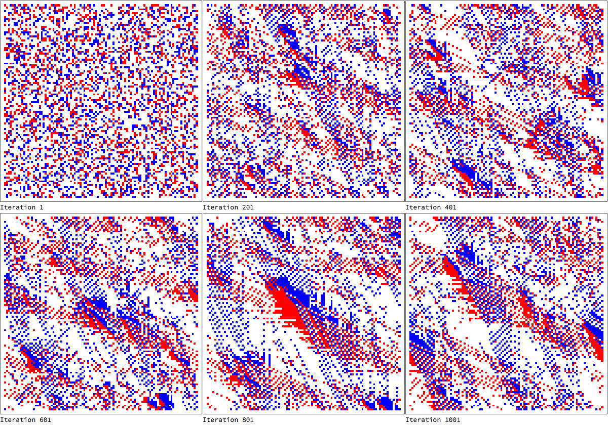
The following code simulates the Biham-Middleton-Levin traffic model for 1000 iterations using explicit rules. According to Wikipedia the blue and red cars take turns to move, which means each step is simpler than what you implemented, however.
- Simulating cellular automata with better performance has been dealt with here and here. (I've contributed to both.)
- Slow as simulating the system may be, visualizing it is even slower! It could be visualized frame by frame with
Dynamic, but the frame rate would drop quickly with larger grids. We cannot get the same performance as WebGL, as you noted. - I don't see any tangible benefit in using
RulePlot, if it could be made to work, for this scenario.
Code (Export may be replaced by ListAnimate):
fill = 0.36;
board = RandomChoice[{1 - fill, fill/2, fill/2} -> {0, 1, 2}, {100, 100}];


red = {
   {{_, _, _}, {1, 0, _}, {_, _, _}} -> 1,
   {{_, _, _}, {_, 1, 0}, {_, _, _}} -> 0,
   {{_, _, _}, {_, x_, _}, {_, _, _}} :> x
   };
blue = {
   {{_, _, _}, {_, 2, _}, {_, 0, _}} -> 0,
   {{_, 2, _}, {_, 0, _}, {_, _, _}} -> 2,
   {{_, _, _}, {_, x_, _}, {_, _, _}} :> x

   };

redStep = CellularAutomaton[red];
blueStep = CellularAutomaton[blue];

evolve[board_] := blueStep[redStep[board]]

frames = NestList[evolve, board, 1000];

imageFrames = MapIndexed[Column[{

      ArrayPlot[#, ColorRules -> {2 -> Blue, 1 -> Red, 0 -> White}, ImageSize -> 400],
      StringTemplate["Iteration ``"]@First[#2]
      }] &, frames];

Export["~/Desktop/traffic.gif", imageFrames]

Just to show you how I might have written you implementation using explicit rules, the two first rules in the Switch statement might've been written like this:
moveInRedComesFirst = {
   {{_, _, _}, {1, 0, _}, {_, _, _}} -> 1,

   {{_, 2, _}, {_, 0, _}, {_, _, _}} -> 2,
   {{_, _, _}, {_, 0, _}, {_, _, _}} -> 0
   };
moveRedLetBlueIn = {
   {{_, _, _}, {2, 1, 0}, {_, _, _}} -> 2,
   {{_, _, _}, {_, 1, 0}, {_, _, _}} -> 0,
   {{_, _, _}, {_, 1, _}, {_, _, _}} -> 1
   };
The order of the rules encode the If statements in a natural way; if the first rule doesn't match, it will proceed to the second one, and so on. The complete ruleset would be combination of these two and the third rule:
Join[moveInRedComesFirst, moveRedLetBlueIn, moveBlueIfRoomNoRedComingOrGoing]
Comments
Post a Comment